This blog post is part of a series summarising my PhD project and the steps to complete my degree. The information in this blog post discusses the modelling and fabrication process outlined in Chapter 4 used to create a gripper prototype. Refer to thesis for full details.
Introduction
In the previous blog post, an inspired conceptual gripper design was found. Now, the next stage of my PhD involved creating a gripper prototype inspired by lateral grasping and a simulated model. The development process, a journey of innovation and perseverance, included using classical mechanics, fabrication techniques, and engineering practices to iteratively create the manipulator. This resulted in a simulated URDF model and a hardware prototype. The development process involved multiple redesigns and testing before arriving at a final prototype revision.
The various iterations are shown below. The gripper developed is a serial link structure with a single prismatic actuator moving along a rail. At the same time, a thumb appendage comprises rotation actuators that move along the rail to form grasps. While most of the lateral grasp can be represented by rotation actuators, which represent the thumb, the rail component exists to account for motion in the index finger, an issue highlighted in the previous post. Two-fingered grasps are formed by pressing the end of the serial-link thumb structure into a static plate mounted to gripper’s chassis.
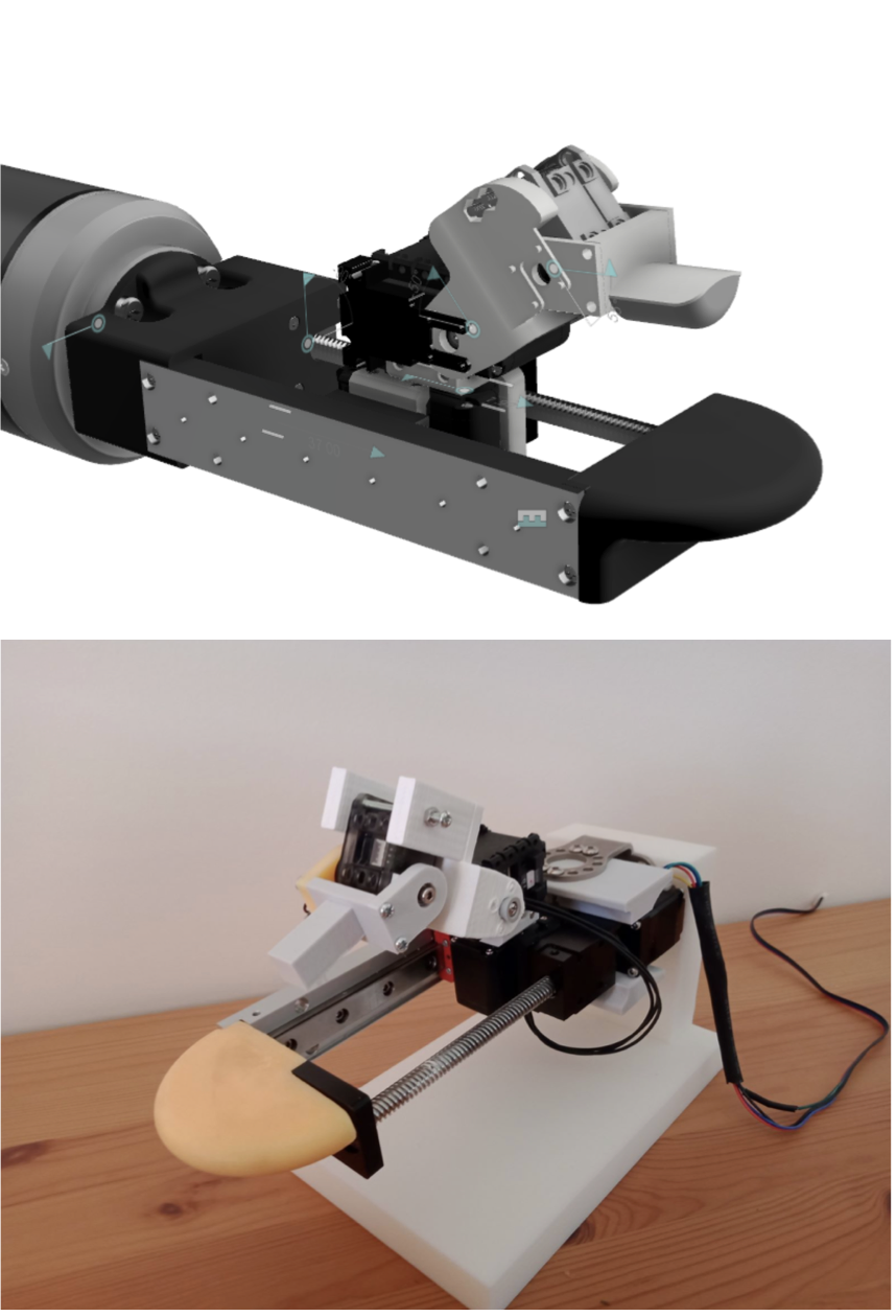
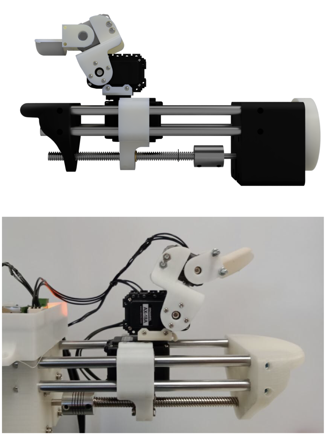
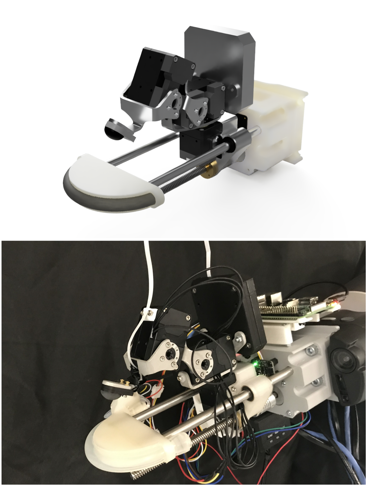
The various hardware prototypes developed before reaching the final research prototye (on the right).
The final research prototype was equipped with the Dynamixel XM-430-350-R actuators, which operated the rotational joints. These actuators’ vital benefit is their built-in position controllers with impedance features, which enable grasp force modulation. A stepper motor, coupled with a ball-screw mechanism, provided the necessary linear motion of the prismatic actuator. These actuation choices were made after carefully considering the gripper’s requirements and the available technologies at the time.
Two critical sensors are included in the final design iteration, along with the actuation elements. The first sensor is a tri-axial force sensor embedded in the fingertip of the gripper. This sensor is provided by Contactile. It consists of a rubber body with a pinhole camera and quadrant photo-diode embedded in the base. Inside the rubber body, there is a diffuse reflector with illumination LEDs. As contact occurs, the rubber body moves and deforms, causing a shift in the positioning of the diffuse reflector. Simultaneously, the photo-diode reads light data from the diffuse reflector.
The pressure sensor is the second sensor, and it evaluates readings in an airtight silicon tube located at the end of the static plate appendage. This sensor provides a signal to indicate when the manipulator makes contact with the environmental surface. The silicon tube, which has an attached pressure sensor, gives feedback to the gripper system. It detects rigid object collisions with the static plate by sensing changes in pressure when the tube deforms. This component serves a crucial function of continuously detecting forces applied to the static plate when attempting to grasp flattened clothing. The sensors and actuators can be seen in the visualisation below.
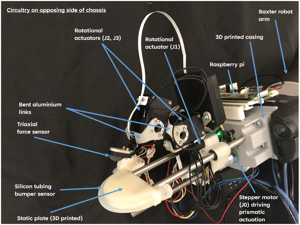
Overview of gripper with labelled components.
Modelling
Initial Definitions
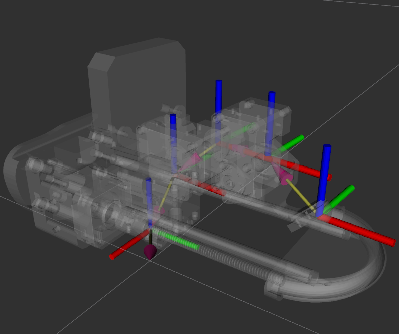
However, before fabrication, the modelling must be outlined first. The serial-link structure of the proposed gripper can be represented by the Denavit-Hartenberg (DH) parameters. The exact details surrounding the DH parameters can be found in the thesis. However, the defined parameters resulted in the Kinematic diagram shown below, where the blue coordinate frame represents the gripper’s base frame, and the red frame outlines the tool-center point (TCP) of the structure.
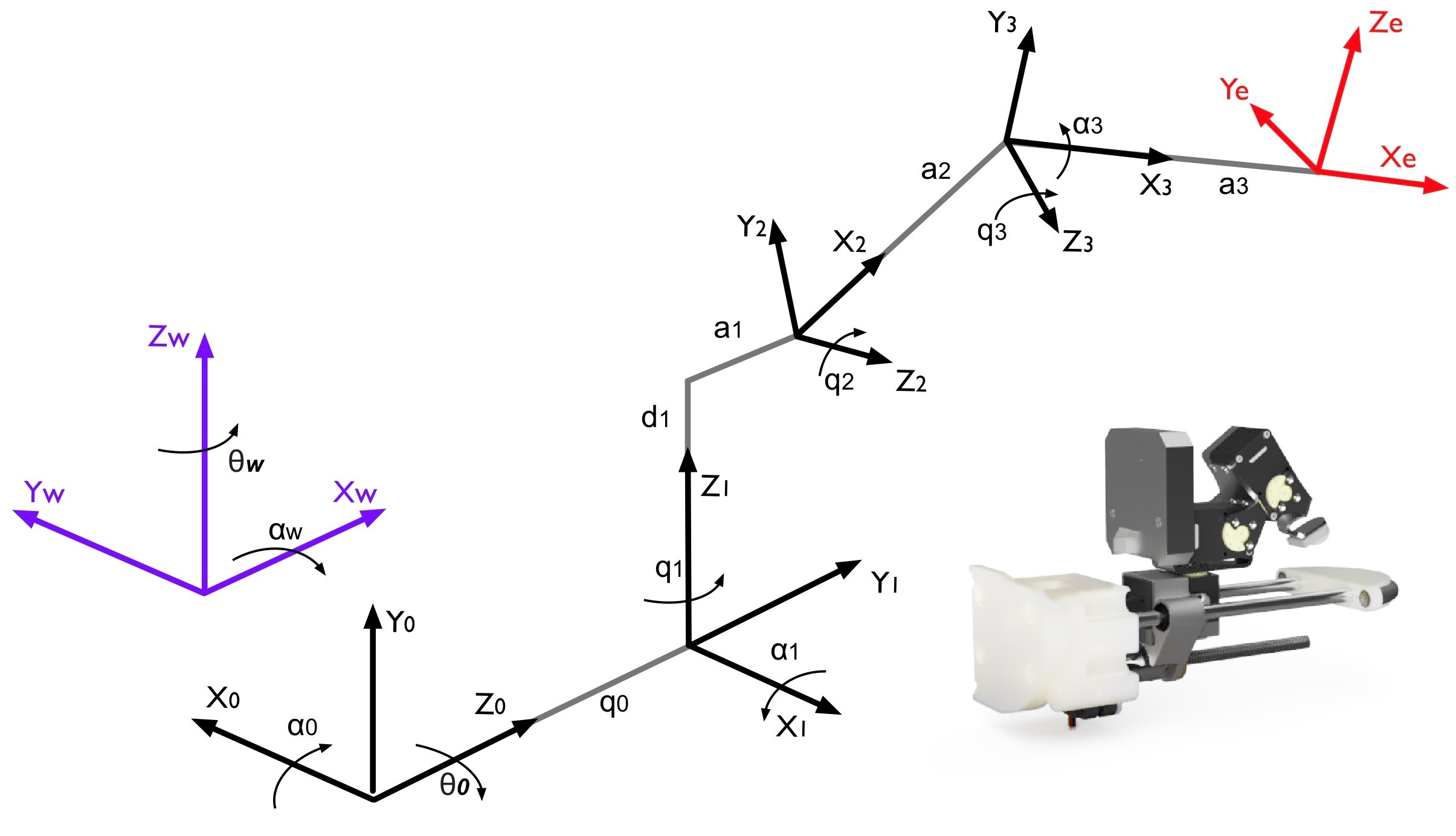
Kinematic diagram of proposed gripper.
In addition, when defining the DH parameters, one also defines the range of motion for each actuator, as the image below displays.
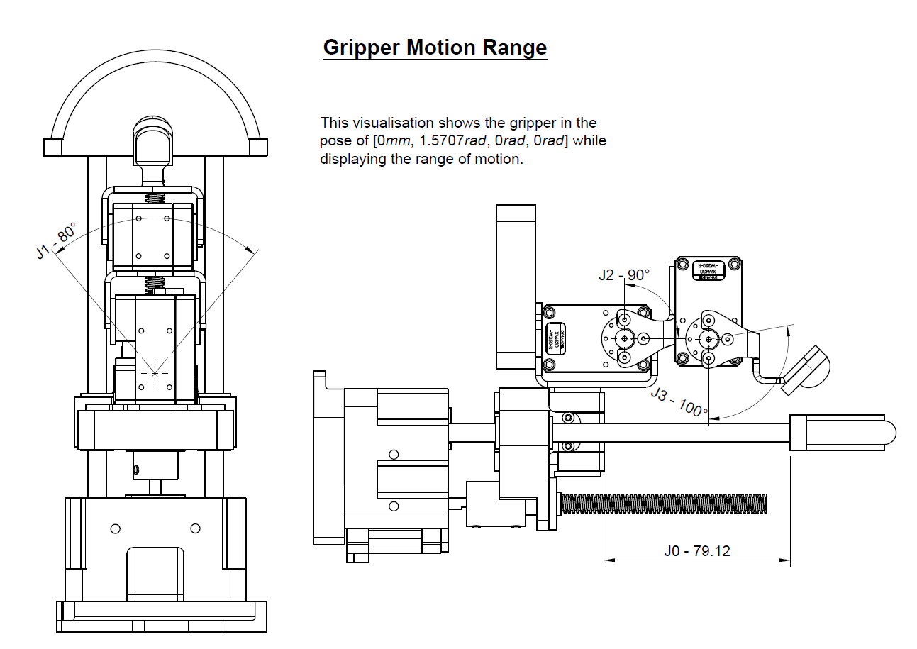
Mechanical drawing highlighting the griper's range of motion.
Forward Kinematics
To represent the closed-form kinematics solution, a set of equations that relate the base and TCP position, both from base to TCP (forward kinematics, FK) and vice-versa (inverse kinematics, IK). Note that these equations use variables like \(a_{i}\) or \(d_{i}\) refering to constants in the DH parameters. The actuator position variables \(q_{i}\) are used to establish the FK equations, which calculate the TCP's position relative to the base.
$$ x = q_{0}+\sin\left(q_{1}\right)\,\left(a_{1}+a_{3}\,\cos\left(q_{2}+q_{3}\right)+a_{2}\,\cos\left(q_{2}\right)\right) $$ $$ y = -\cos\left(q_{1}\right)\,\left(a_{1}+a_{3}\,\cos\left(q_{2}+q_{3}\right)+a_{2}\,\cos\left(q_{2}\right)\right) $$ $$ z = d_{1}+a_{3}\,\sin\left(q_{2}+q_{3}\right)+a_{2}\,\sin\left(q_{2}\right) $$ $$ p = -q_{2}-q_{3} $$
Inverse Kinematics
Alternatively, the IK calculates the actuator positions using the x, y, and z position variables and the pitch or rotation of the y-axis of the TCP (relative to the base).
$$ q_0 = x-\sin\left(q_{1}\right)\,\left(a_{1}+a_{3}\,\cos\left(q_{2}+q_{3}\right)+a_{2}\,\cos\left(q_{2}\right)\right) $$ $$ q_1 = \pi -\mathrm{acos}\left(\frac{y}{a_{1}+a_{3}\,\cos\left(q_{2}+q_{3}\right)+a_{2}\,\cos\left(q_{2}\right)}\right) $$ $$ q_2 = \mathrm{asin}\left(\frac{z - d_1 + a_3sin(p)}{a_2}\right) $$ $$ q_3 = -p-q_{2} $$
Before concluding this section, it is worth noting that the set of equations is simply the closed-form solution of the kinematics for the DH parameters; however, when the fingertip sensor component is placed into the gripper design, an alternative set of both kinematic and kinostatic equations can be found in the thesis. This parallel modelling component is needed to account for minor differences in the sensor’s position compared to the traditional DH parameter’s TCP.
Velocity Kinematics
In order to model velocity kinematics, I extended the forward kinematic equations to create a Jacobian matrix. This matrix can establish the relationship between velocity in the base and TCP (tool center point) frame [Corke 17]. The Jacobian matrix is derived from the forward kinematic equations by partially differentiating each expression with respect to the position of each actuator in the system. This results in a matrix that depends on the positions of the actuators (\(q\)). The resulting Jacobian, \(J(q)\)), takes the simplified form shown below.
$$ J(q) =\left\lbrack \begin{array}{cccc} \frac{\partial x}{\partial q_0 } & \frac{\partial x}{\partial q_1 } & \frac{\partial x}{\partial q_2 } & \frac{\partial x}{\partial q_3 }\\ \frac{\partial y}{\partial q_0 } & \frac{\partial y}{\partial q_1 } & \frac{\partial y}{\partial q_2 } & \frac{\partial y}{\partial q_3 }\\ \frac{\partial z}{\partial q_0 } & \frac{\partial z}{\partial q_1 } & \frac{\partial z}{\partial q_2 } & \frac{\partial z}{\partial q_3 }\\ \frac{\partial p}{\partial q_0 } & \frac{\partial p}{\partial q_1 } & \frac{\partial p}{\partial q_2 } & \frac{\partial p}{\partial q_3 } \end{array}\right\rbrack $$
When calculated, \(J(q)\) becomes:
$$ \left(\begin{array}{cccc} 1 & \mathrm{c}\left(q_{1}\right)\,\left(a_{1}+a_{3}\,\mathrm{c}\left(q_{2+3}\right)+a_{2}\,\mathrm{c}\left(q_{2}\right)\right) & -\mathrm{s}\left(q_{1}\right)\,\left(a_{3}\,\mathrm{s}\left(q_{2+3}\right)+a_{2}\,\mathrm{s}\left(q_{2}\right)\right) & -a_{3}\,\mathrm{s}\left(q_{2+3}\right)\,\mathrm{s}\left(q_{1}\right)\\ 0 & \mathrm{s}\left(q_{1}\right)\,\left(a_{1}+a_{3}\,\mathrm{c}\left(q_{2+3}\right)+a_{2}\,\mathrm{c}\left(q_{2}\right)\right) & \mathrm{c}\left(q_{1}\right)\,\left(a_{3}\,\mathrm{s}\left(q_{2+3}\right)+a_{2}\,\mathrm{s}\left(q_{2}\right)\right) & a_{3}\,\mathrm{s}\left(q_{2+3}\right)\,\mathrm{c}\left(q_{1}\right)\\ 0 & 0 & a_{3}\,\mathrm{c}\left(q_{2+3}\right)+a_{2}\,\mathrm{c}\left(q_{2}\right) & a_{3}\,\mathrm{c}\left(q_{2+3}\right)\\ 0 & 0 & -1 & -1 \end{array}\right) $$
To use \(J(q)\), variables defining the velocities of the actuators and TCP positions are defined with dots above the respective position variables. Then, using these parameters, we can apply both \(J(q)\) and its inverse, as shown in the two expressions below, to define the velocity relationship between the TCP and actuators.
$$ \left\lbrack \begin{array}{c} \dot{x} \\ \dot{y} \\ \dot{z} \\ \dot{p} \end{array}\right\rbrack =J(q)\dot{q} \;=\;J(q)\left\lbrack \begin{array}{c} \dot{q_0 } \\ \dot{q_1 } \\ \dot{q_2 } \\ \dot{q_3 } \end{array}\right\rbrack $$
$$ \dot{q} \;=J(q)^{-1} \left\lbrack \begin{array}{c} \dot{x} \\ \dot{y} \\ \dot{z} \\ \dot{p} \end{array}\right\rbrack $$
Before proceeding to the Kinostatics, it's essential to calculate the determinant using the Jacobian matrix. In the context of serial manipulation design, when the determinant of a Jacobian matrix equals 0. The system encounters a kinematic singularity, meaning the Jacobian loses rank and calculations using \(J(q)\) will fail. In the case of this system, this situation occurs under one scenario in which \(q_{2}\) is equal to \(\frac{\pi}{2}\). When such a circumstance arises, an easy solution is to add a small amount of noise to the position of \(q_{2}\), enabling the Jacobian matrix to operate across the manipulator workspace.
Kinostatics
Kinostatic methods provide the relationship between the wrench exerted at the TCP frame based on the actuator forces and torques. This modelling section is quite simple when building upon the velocity kinematics outlined in the previous section. First, the forces and torques exerted by the actuators are represented by \(\tau_i\). Next, the forces (\(f_i\)) and moments (\(m_i\)) at the TCP's wrench are defined. Finally, the transpose of \(J(q)\) is taken, \(J(q)^T\), and can be used alongside its inverse to map the relationship between the actuator's forces/torques to the wrench exerted at the TCP. Note that this relationship will not account for system motion, calculated with the dynamics analysis .
$$ \left\lbrack \begin{array}{c} \tau_0 \\ \tau_1 \\ \tau_2 \\ \tau_3 \end{array}\right\rbrack ={J\left(q\right)}^T \left\lbrack \begin{array}{c} f_x \\ f_y \\ f_z \\ m_y \end{array}\right\rbrack $$
$$ \left\lbrack \begin{array}{c} f_x \\ f_y \\ f_z \\ m_y \end{array}\right\rbrack ={(J\left(q\right)}^T)^{-1} \left\lbrack \begin{array}{c} \tau_0 \\ \tau_1 \\ \tau_2 \\ \tau_3 \end{array}\right\rbrack $$
Dynamics
The final component of the modelling is the dynamics. Simply put, the dynamics analysis is the modelling that establishes the relationship between the actuator's forces and torques \(\tau\) and their respective position \(q\), velocity \(\dot{q}\), and acceleration \(\ddot{q}\). The inverse dynamics formulation maps desired motion to actuator forces \(q, \dot{q}, \ddot{q}\to \tau\) while considering dynamic parameters like inertia, mass and gravity. The inverse dynamics of a serial link manipulator can be succinctly expressed in the following equation. In this equation, \(M(q)\) represents the inertia experienced by each joint and the products of inertia between joints. \(C(q, \dot{q})\) is a function of the manipulator's current velocity and position, providing information about the centripetal torques caused by each joint and the Coriolis torques produced by joint pairs. Finally, \(G(q)\) contains information about the forces required to overcome gravity in the manipulator's current configuration.
$$ \tau = M(q)\ddot{q} + C(q,\dot{q})\dot{q} + G(q) \label{Eq::ConsiseDynamics} $$
The Lagrangian, expressed below, can be described as the difference between potential energy \(\mathcal{U}\) and kinetic energy \(\mathcal{T}\), or \(\mathcal{L} = \mathcal{T} - \mathcal{U}\). According to definitions provided by [Yoshikawa 90] and Sciavicco and Siciliano [Sciavicco 12], the first expression represents the torque or force required at each actuator. The alternative form in the second expression is also acceptable.
$$ \begin{equation} \tau_{i} =\frac{d}{\mathrm{d}t}\left(\frac{\partial }{\partial \dot{q_i } }\mathcal{T}\right)-\frac{\partial }{\partial q_i }\mathcal{T}+\frac{\partial }{\partial q_i }\mathcal{U} \label{Eq::LagragianExpressionForEachActuator} \end{equation} $$ $$ \begin{equation} \tau_i =\frac{d}{\mathrm{d}t}\left(\frac{\partial }{\partial \dot{q_i } }\mathcal{L}\right)-\frac{\partial }{\partial q_i }\mathcal{U} \label{Eq::LagragianExpressionForEachActuatorAlt} \end{equation} $$
The complete dynamics calculation is a tedious process, which would double the length of this post, so it's not included for brevity's sake. However, for the interested reader, the thesis has all the excellent nitty-gritty details. As someone with a software background, it was definitely a challenge to get my head around the dynamics calculation, but I found it to be a profound experience that gave me a deeper insight and appreciation for the mechanical knowledge needed to use robots.
Wrapping up
This section has shown a broad approach to modelling the gripper. However, this post omits these extended modelling elements for brevity and encourages readers to examine the thesis for such details. Examples include the calculations for translating the torque exerted by the stepper motor to the forces wielded by the ball-screw driven rail. In addition, the dynamics calculation and how it validated actuator choice are also detailed in the thesis. Lastly, the Jacobian matrix method to calculate the manipulator’s grasp force characteristics is also presented. These are a few examples of the considerations one should make when building robotics systems; curious readers can see these details here.
Design and Prototyping
Fabrication
After designing the system, I proceeded with fabricating the proposed manipulator. The first component created was the prismatic rail, which was incorporated into the primary chassis and coupler of the Baxter robot. As shown in the visualisation, a NEMA-17 stepper motor connected to a threaded rod with a lead screw was used to achieve the desired linear motion. Two additional non-threaded rods supported the linear motion. They allowed me to attach the static plate component to the chassis for grasping. This design allowed the thumb appendage to slide closer to the static plate component while establishing a core chassis design as a foundation for further development.
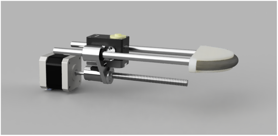
Visualisation of Main Prismatic Rail Components.
The surrounding infrastructure is attached to the gripper following the prismatic rail design. This process involves designing a coupler for attachment to the Baxter robot and the remaining actuator-link pairings. As mentioned earlier, ROBOTIS supplies the Dynamixel XM-430-350-R servo motors for rotational motion. These motors provide the correct motion controller behaviours and feedback, enabling robust operation. Creating the rest of the gripper used multiple fabrication approaches, including 3D printing and bending aluminium sheets. For the coupler, static plate, and minor components, FDM printing was sufficient. However, custom-bent aluminium parts were better suited for the components forming grasps with the gripper for the links connecting the rotational actuator mechanisms. In addition, the silicon tube making up the pressure environment collision sensor was also embedded into the end of the static plate. These various components can be seen in the exploded image below.
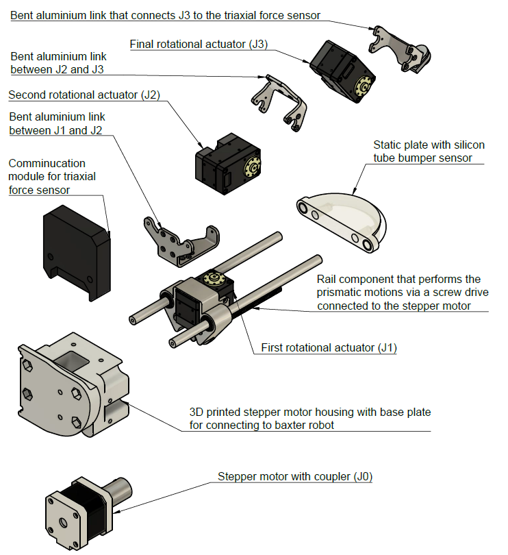
Exploded View of Gripper Design.
The final dimensions of the fabricated research prototype can be seen in the image below.
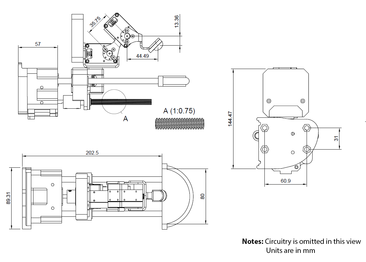
Mechanical Diagram of Prototype with Dimensions.
Simulation
ROS uses Unified Robot Description Format (URDF) XML files to embed simulated robot designs into simulation and visualisation platforms. The 3D modelling program Fusion 360 was initially used to design the gripper. Using a publicly available plugin, I could set the physical material properties of the various components and export a URDF with the broadly correct dynamic parameters, including the centre of mass, inertia tensor, and weight of each joint-link pair of the robotic system. I could use these values to evaluate my dynamics model formulated via the Lagrangian by plugging in this information and evaluating the required forces for various gripper motions and positions. Such a step is shown in the thesis, validating that my actuator selection was valid for the intended use cases.
###.
In addition to validating the dynamics model of my gripper, building the URDF also set my research for the last research contribution of my thesis, which trained the gripper in simulation to perform grasping motions that leveraged the environment. However, this process will be detailed in the next post of this series.
Implementing the Electronics
I made a custom circuit board and communication protocol to control the actuators and communicate the robot manipulator’s current state. This allowed us to maintain control of the robot and reliably communicate with the host ROS system. The Dynamixel XM-430-350-R actuators use the RS-485 protocol to communicate with a serial interface. A max485 chip is connected to the microcontroller’s serial line (TX/RX pins). The microcontroller then utilized a library provided by the manufacturer to communicate with the servomotors across the serial line. Communicating with these actuators involved sending the commands for a desired goal position and current/torque. Information received included the present velocity, position, temperature, etc.
Controlling the prismatic actuator with a stepper motor was a bit more complicated. Unlike the rotational actuators, there were no built-in controllers. Therefore, a custom controller that accepts desired position and velocity commands was implemented. An A4988 breakout circuit interfaced with an ATmega32U4-driven microcontroller to integrate the stepper motor with the electronics. The microcontroller then pulsed the stepper motor based on whether the actuator was at the target position, and a target velocity determined the pulsing speed. The ATmega32U4 device (known as the Qwiic Pro microcontroller) also acted as the controller and processed commands via serial to set the target speed and position, while providing feedback on the present motion details. One limitation of this approach is that controlling the stepper motor component in this manner remains an open-loop system. This description is appropriate as there is no mechanism to validate that steps have pulsed successfully, i.e., not skipping steps. To somewhat address this a limitation, a laser measuring the linear displacement of the rail was present for calibration routines during operation.
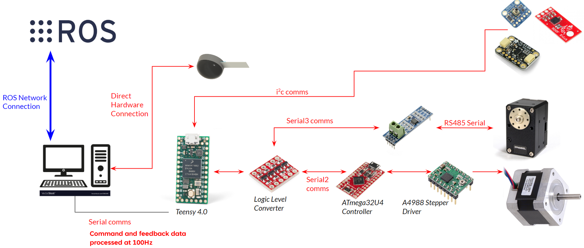
An overview of the system electronics.
The primary communication device was a Teensy 4.0 microcontroller. It sent serial data to the Dynamixels and the microcontroller operating the stepper-driven rail. The Teensy also communicated with the host PC through another serial line that was responsible for controlling the manipulator’s commands and receiving feedback data. In addition, several sensors interfaced with the Teensy microcontroller using the i2c bus. These sensors provided additional feedback information, including the manipulator’s orientation through an inertial measurement unit (IMU), detecting collisions with the environment using a pressure sensor and determining the position of the prismatic actuator with a time-of-flight (ToF) laser.
The inertial measurement unit (IMU) device was connected to the I2C bus on the printed circuit board (PCB) attached to the hand. The pressure sensor evaluated readings in an airtight silicon tube at the end of the static plate appendage. This mechanism provided a signal to indicate if the manipulator had made contact with a rigid workspace surface. Finally, the manipulator used the ToF laser embedded in a position that enabled it to query the displacement of the rail component if required. However, the ToF laser takes over 100ms to collect a single reading. Therefore, during operation, a ToF reading only occurs upon request, and system serial communication is paused. Such a solution is useful for calibrating the rail component. Still, it cannot enable closed-loop operation for the prismatic rail and stepper motor.
Integrating into ROS
Due to lab constraints at the time, I had to integrate the gripper on the Baxter robot (see the video at the end of this article) to evaluate the procedure and create a demo. This involved developing the software framework under the ROS1 Indigo distro (despite ROS2 Foxy being out then). Several weekends were spent reviewing the documentation, and several software adjustments were required to operationalise the system. However, no challenge was too bad, and these efforts are usually a part of developing robotic systems; you’ll always have to make concessions or work with the hardware you have available.
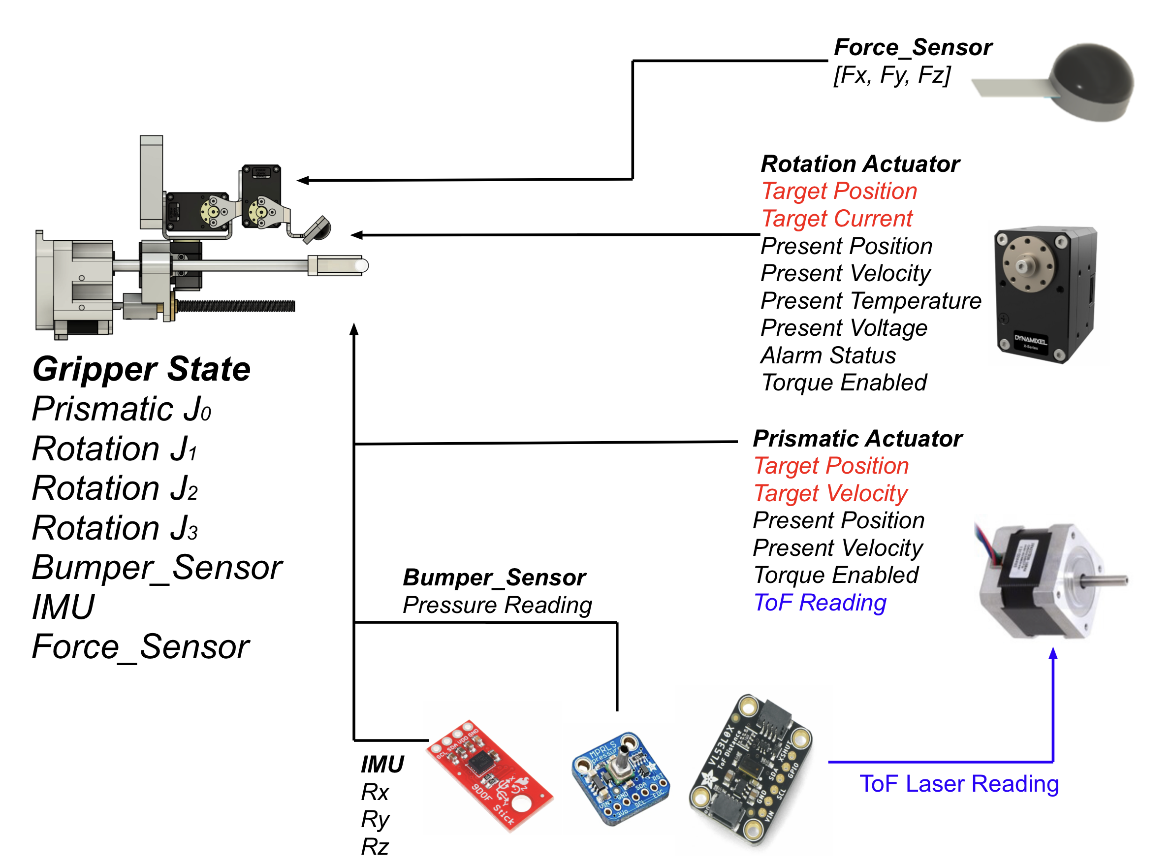
Several modules had to be developed throughout this process, including reactive trajectories for Baxter motion, the gripper drivers, ROS communication channels, computer vision modules to detect garments, and services/actions to integrate evaluation procedures. However, much of this development process never made it into the final thesis. Which is a little frustrating and demonstrates the sheer amount of background work needed to complete a robotic system from start to scratch. To show how the gripper component was integrated into the system. The image below shows the ROS message framework for the gripper’s actuators and sensors. These variables were obtained by the various drivers and their respective ROS interfaces. While interfacing with Python programs across the ROS network for broader services and actions, the complete system could operate at over 33Hz.
###.
Initial Evaluation
While developing the gripper, the preliminary design and evaluation were published at the 2020 Conference of Automation Science and Engineering (CASE) [Hinwood 20]. This publication presented the first design iteration of the gripper. It demonstrated grasping from the environment alongside the initial kinematic modelling process. However, this first design used actuators that were only capable of position and velocity control; thereby, they were not suited for long-term grasping applications but were helpful for early-stage demonstrations, as shown in the videos below.
In the thesis, several evaluation procedures are carried out. First, the Kinostatic model estimates the theoretical grasp forces compared to the real-world characteristics of the grasping devices. When evaluating the final research prototype, it was discovered that the gripper could exert a maximum grasping force of 29 newtons, which was close enough to the recommended 30 newtons for general manipulation [Le 13].
The prototype’s grasp force characteristics were lower than the Jacobian estimations. Upon further investigation, some minor issues were noted, including mechanical backlash in the final research prototype design, the rubber body of the TCP sensor potentially impacting force readings, and the load cell used to evaluate grasp forces possibly experiencing a minor deterioration in accuracy. Despite these considerations, the prototype’s grasp force was sufficient to move forward.
In addition to evaluating the grasp force, I also conducted a process to assess the final research prototypes’ grasp strength in a practical setting. This involved testing the gripper’s ability to hold various textile materials with additional weights to demonstrate its capability to hold different garment payloads despite the complex interplay of friction and applied grasp force. Inspired by an experiment by Donaire et al. [Donaire 20], the gripper would hold clothing for 20 seconds with a varying amount of additional weight applied.
The set of garments evaluated in this trial included a jumper, necktie, jean shorts, scarf, and t-shirt, as shown in the images below. When exerting the maximum available torque, the gripper could hold all garments regardless of the garment and additional weight applied. This evaluation’s most extreme garment weight was 1050g (while holding the jumper with the additional 550g), which was still an easy task for the real-world prototype.
The evaluation procedure in which the gripper held various garments with weights.

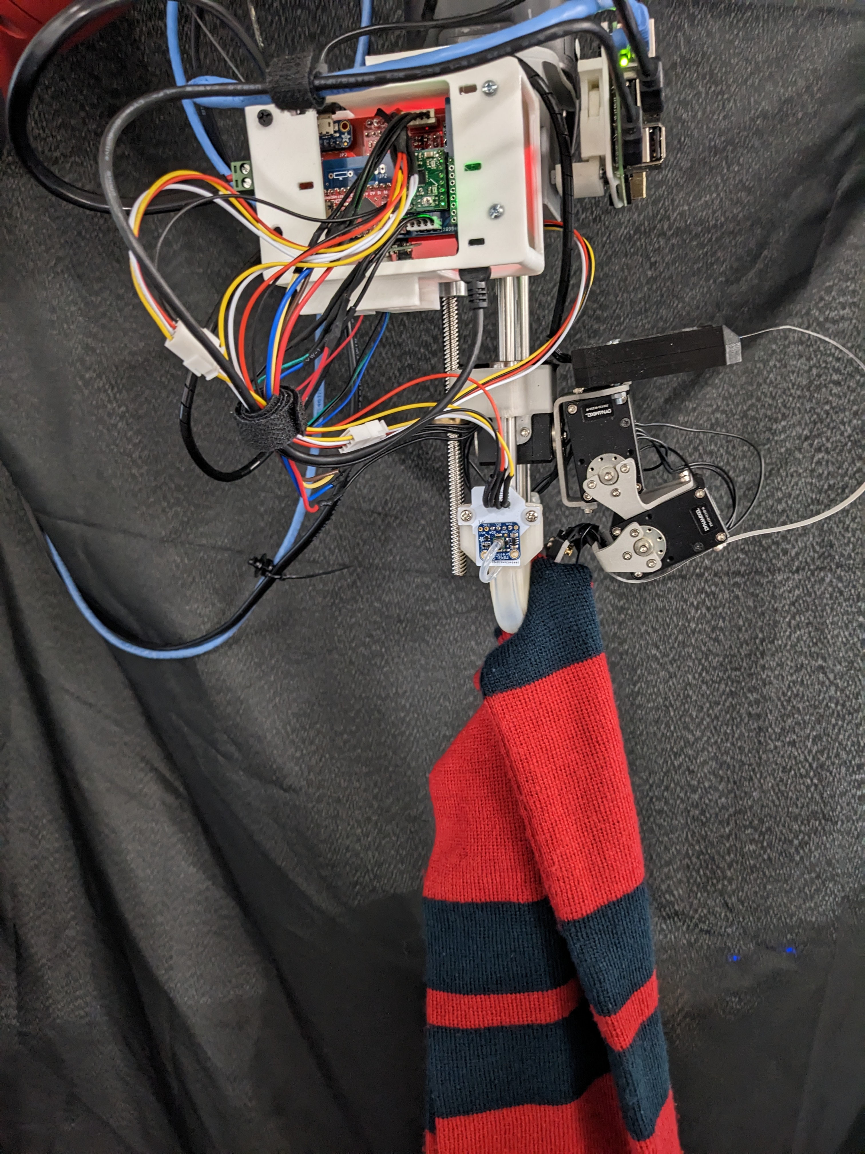
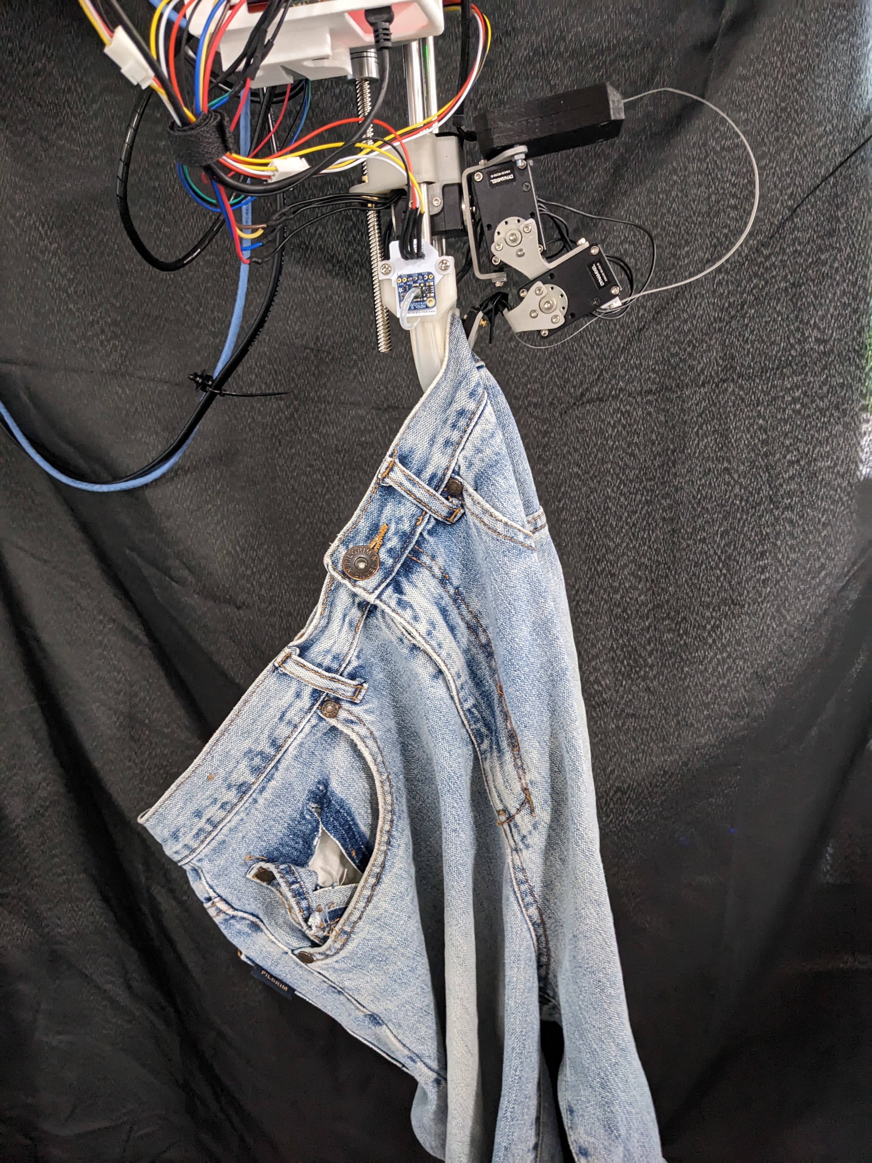
Holding a Shirt Holding a Scarf Holding Jean Shorts
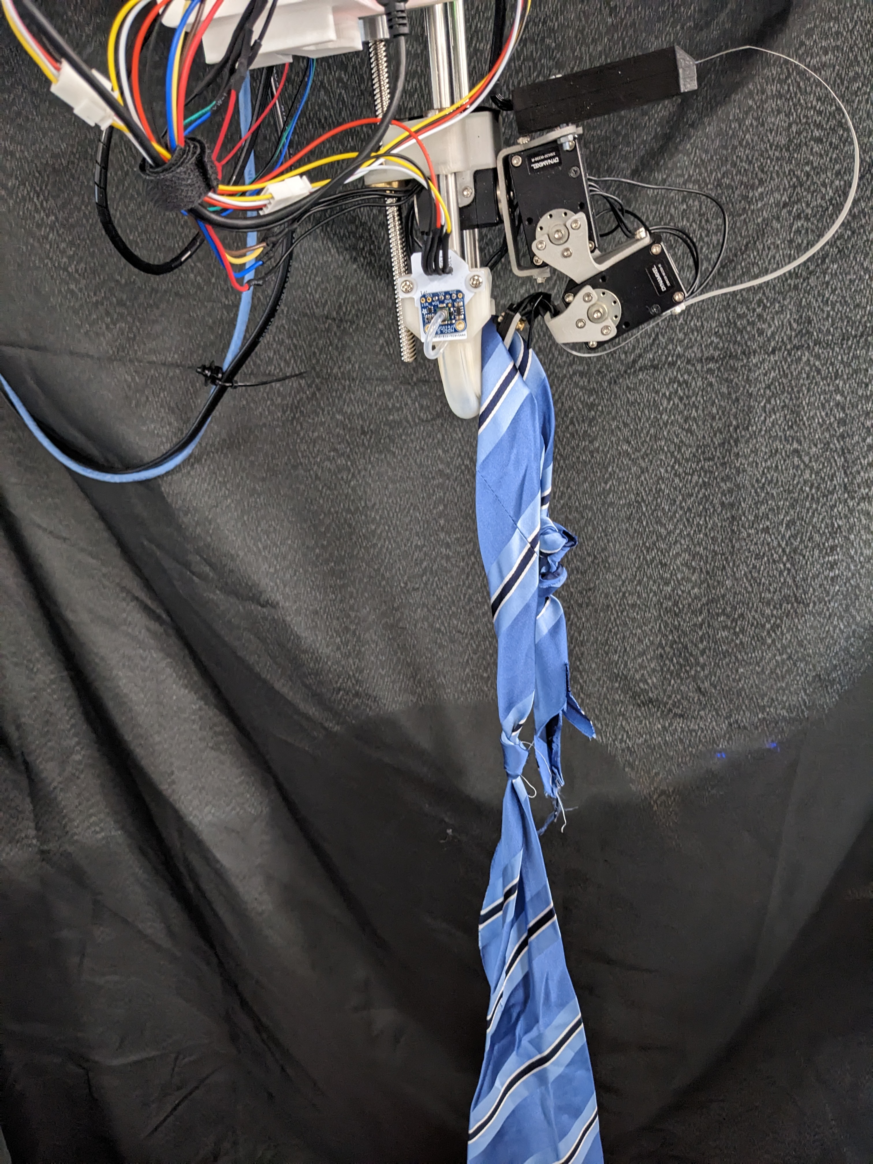
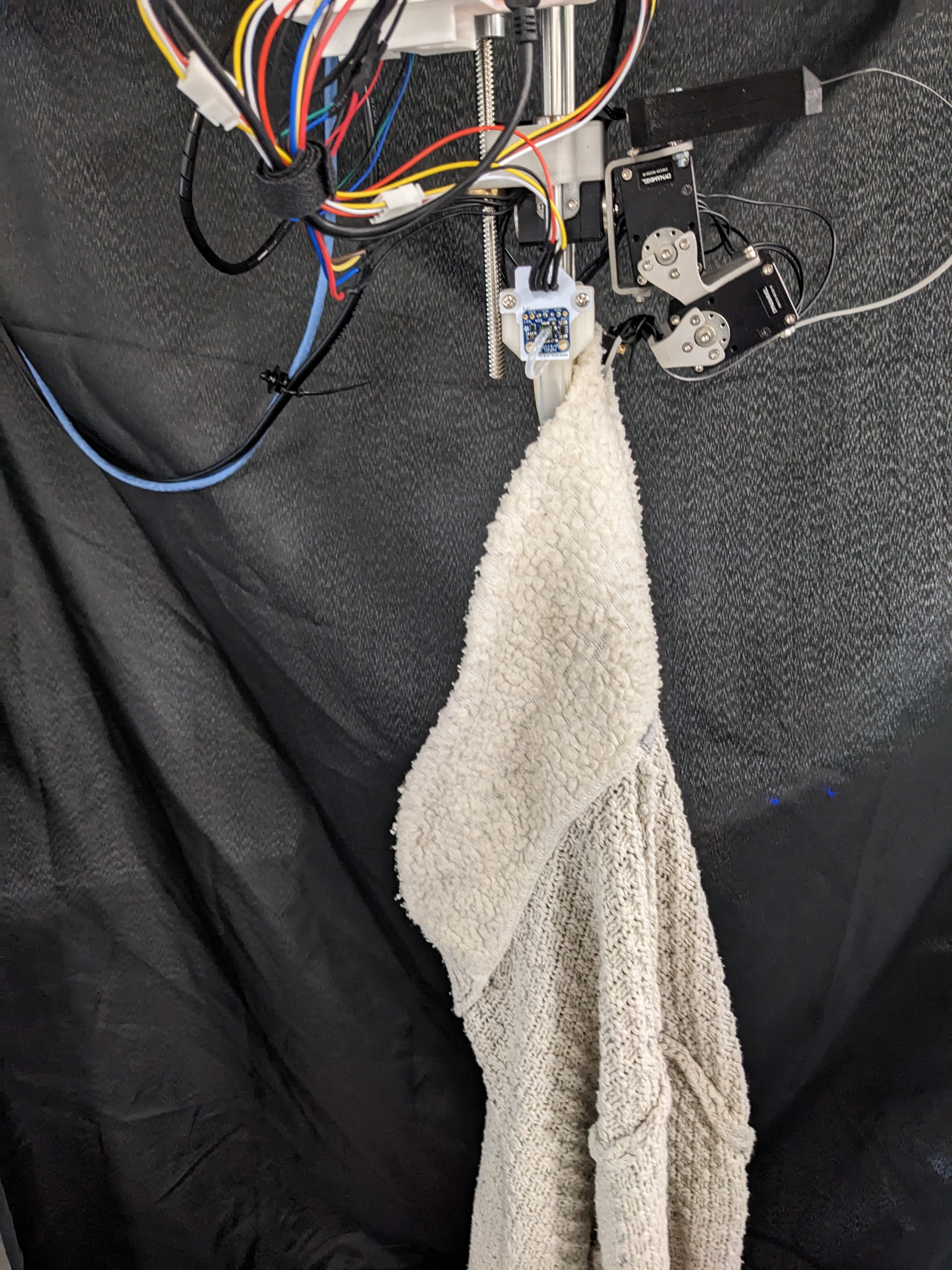
Holding a Necktie Holding a Jumper
After Development
Having completed the modelling, fabrication, and evaluation process described above, the conceptual gripper design described in the previous post has been developed as a simulated model and a hardware prototype. The gripper uses existing serial-link modelling processes [Corke 17, Yoshikawa 90]. Additionally, the device can modulate grasp force and apply appropriate grasping forces required for general fabric manipulation. It also addresses the previously mentioned limitation of being able to perform grasps from various wrist orientations while grasping and navigating environmental constraints. These features contribute to the unique nature of this general pick-and-place fabric sorting solution.
Compared to previous solutions, the presented gripper remained the only solution at the creation time capable of simultaneously performing haptic exploration, grasp gaiting, grasp force modulation and biomimetic grasping motions. Due to time constraints, some of these skills were not explored in my thesis and require further investigation. While the gripper in its present form has some limitations, it fulfils the outlined requirements by presenting a serial-link gripper that retains the capabilities for pick-and-place sorting of textile waste. The finalised prototype is sufficient to investigate the last area of my thesis, which applies deep reinforcement learning algorithms upon the gripper to learn collision-rich grasping motions.
An early test with a simple instance segmentation model detection clothing and the baxter robot moving to grasp the clothing with the final research prototype integrated.
References
Use this link to view the next post surrounding my PhD project. This next post applies reinforcement learning techniques to use the gripper to grasp flattened clothing while leveraging environmental constraints.